40. Simple linear regression

Correlation (§2) measures whether two variables move together. Regression goes further: it fits an explicit equation, so you can predict one variable from the other and quantify how much each unit of x is worth.

The model

Y_i = \beta_0 + \beta_1 x_i + \varepsilon_i

• \beta_0 — the intercept: the mean of Y when x = 0.
• \beta_1 — the slope: the mean change in Y per one-unit increase in x.
• \varepsilon_i — the error: everything the line doesn't explain.

The standard assumptions on the errors:

E[\varepsilon_i] = 0, \qquad \operatorname{Var}(\varepsilon_i) = \sigma^2, \qquad \varepsilon_i \text{ independent}

Constant variance is called homoscedasticity. Normality of \varepsilon is not needed for the estimates themselves — only for exact inference in small samples.

Note what is and isn't random. x is treated as fixed; the randomness lives entirely in \varepsilon, and hence in Y. The model describes the conditional distribution:

E[Y \mid x] = \beta_0 + \beta_1 x

which is exactly the conditional mean of a bivariate Normal from §2 — this is where the linearity comes from when the data really is jointly Normal.

Least squares

Choose \hat\beta_0, \hat\beta_1 to minimise the sum of squared residuals:

S(\beta_0, \beta_1) = \sum_{i=1}^n \big(y_i - \beta_0 - \beta_1 x_i\big)^2

Setting both partial derivatives to zero gives the normal equations, and solving them:

\hat\beta_1 = \frac{\sum(x_i - \bar x)(y_i - \bar y)}{\sum(x_i - \bar x)^2} = \frac{S_{xy}}{S_{xx}} = r\frac{s_y}{s_x}

\hat\beta_0 = \bar y - \hat\beta_1\bar x

Three things worth noticing:

The slope is the correlation, rescaled. \hat\beta_1 = r\,s_y/s_x — same information, different units. r is dimensionless; \hat\beta_1 is in units of y per unit of x.

The line always passes through (\bar x, \bar y). That's what the intercept formula says.

Why squared errors? Partly because it gives a closed form. But more substantially: if \varepsilon \sim N(0, \sigma^2), then minimising the squared error is maximum likelihood (§4) — the log-likelihood contains -\frac{1}{2\sigma^2}\sum(y_i - \beta_0 - \beta_1x_i)^2 and nothing else that depends on \beta.

Regression to the mean

Since \hat\beta_1 = r\,s_y/s_x, predictions in standardised units are

\frac{\hat y - \bar y}{s_y} = r \cdot \frac{x - \bar x}{s_x}

Because |r| \le 1, the prediction is always closer to the mean, in standard units, than the input was. A student two standard deviations above average on the first test is predicted to be only 2r above on the second.

This is not a force pulling things toward mediocrity — it's a consequence of imperfect correlation. It's also the phenomenon Galton named, giving regression its otherwise puzzling name.

Inference on the slope

\operatorname{Var}(\hat\beta_1) = \frac{\sigma^2}{S_{xx}}, \qquad \widehat{\operatorname{SE}}(\hat\beta_1) = \frac{\hat\sigma}{\sqrt{S_{xx}}}

where \hat\sigma^2 = \frac{1}{n-2}\sum e_i^2, with e_i = y_i - \hat y_i the residuals. The n - 2 is two estimated parameters costing two degrees of freedom.

To test H_0: \beta_1 = 0 (no linear relationship):

t = \frac{\hat\beta_1}{\widehat{\operatorname{SE}}(\hat\beta_1)} \sim t_{n-2}

Notice S_{xx} in the denominator of the variance: spreading your x values further apart makes the slope more precisely estimated. Two clusters of points far apart pin down a line better than the same number of points bunched together — which is a genuine experimental design principle.

R-squared

R^2 = \frac{SS_{\text{reg}}}{SS_{\text{tot}}} = 1 - \frac{SS_{\text{res}}}{SS_{\text{tot}}}

The proportion of variance in y explained by the model. For simple linear regression, R^2 = r^2 exactly.

What R^2 does not tell you:

• Whether the relationship is linear. A perfect parabola can give a low R^2.
• Whether the model is correct. Anscombe's quartet is four datasets with identical R^2, slope, and means — and wildly different shapes.
• Whether predictions are useful. That depends on \hat\sigma, in the units you care about.
• Anything about causation.

Always plot the data and the residuals.

Worked example

Hours studied vs exam score, 5 students:

x (hours)	2	3	5	7	8
y (score)	65	70	75	85	90

\bar x = 5, \bar y = 77.

S_{xx} = (2-5)^2 + (3-5)^2 + 0 + (7-5)^2 + (8-5)^2 = 9 + 4 + 0 + 4 + 9 = 26

S_{xy} = (-3)(-12) + (-2)(-7) + (0)(-2) + (2)(8) + (3)(13) = 36 + 14 + 0 + 16 + 39 = 105

\hat\beta_1 = \frac{105}{26} \approx 4.038, \qquad \hat\beta_0 = 77 - 4.038(5) \approx 56.81

\hat y = 56.81 + 4.04x

Interpretation: each additional hour of study is associated with about 4 extra points.

The intercept, 56.81, is the predicted score for zero hours. It sits outside the observed range of x (2 to 8), so it's an extrapolation and shouldn't be taken too seriously — a common trap when intercepts are reported without comment.

Prediction at x = 6: \hat y = 56.81 + 4.04(6) \approx 81.04.

Is the slope significant? The residuals give SS_{\text{res}} \approx 5.96, so \hat\sigma^2 = 5.96/3 \approx 1.99 and \hat\sigma \approx 1.41.

\operatorname{SE}(\hat\beta_1) = \frac{1.41}{\sqrt{26}} \approx 0.277, \qquad t = \frac{4.038}{0.277} \approx 14.61

With df = 3 and t_{3,\,0.025} = 3.182, this is clearly significant (p \approx 0.0007).

And the causal caveat: this shows association. Motivated students may both study more and score higher for reasons unrelated to study time. Nothing in the arithmetic distinguishes the two.

Doing it in Python

From the formulas, then with SciPy:

import numpy as np
from scipy.stats import linregress

x = np.array([2, 3, 5, 7, 8], dtype=float)
y = np.array([65, 70, 75, 85, 90], dtype=float)

# By hand
Sxx = ((x - x.mean()) ** 2).sum()
Sxy = ((x - x.mean()) * (y - y.mean())).sum()
b1 = Sxy / Sxx
b0 = y.mean() - b1 * x.mean()
print(f"by hand : intercept {b0:.4f}  slope {b1:.4f}")

# With SciPy
res = linregress(x, y)
print(f"scipy   : intercept {res.intercept:.4f}  slope {res.slope:.4f}")
print(f"          r = {res.rvalue:.4f}  R^2 = {res.rvalue**2:.4f}")
print(f"          SE(slope) = {res.stderr:.4f}  p = {res.pvalue:.6f}")

# The slope is just the correlation, rescaled
r = np.corrcoef(x, y)[0, 1]
print(f"\nr * sy/sx = {r * y.std(ddof=1) / x.std(ddof=1):.4f}  == slope")

Residual analysis — always do this before trusting a fit:

import numpy as np
from scipy.stats import linregress

x = np.array([2, 3, 5, 7, 8], dtype=float)
y = np.array([65, 70, 75, 85, 90], dtype=float)

res = linregress(x, y)
fitted = res.intercept + res.slope * x
resid = y - fitted

print(f"{'x':>5} {'y':>7} {'fitted':>9} {'residual':>10}")
for xi, yi, fi, ri in zip(x, y, fitted, resid):
    print(f"{xi:>5.0f} {yi:>7.0f} {fi:>9.3f} {ri:>10.3f}")

n = len(x)
ss_res = (resid**2).sum()
sigma_hat = np.sqrt(ss_res / (n - 2))
print(f"\nSS_res {ss_res:.4f}   sigma_hat {sigma_hat:.4f}")
print(f"residuals sum to {resid.sum():.2e}  (always zero, by construction)")
print(f"R^2 = {1 - ss_res / ((y - y.mean())**2).sum():.4f}")

Anscombe's quartet — the argument for plotting, in numbers:

import numpy as np
from scipy.stats import linregress

anscombe = {
    "I":   ([10,8,13,9,11,14,6,4,12,7,5], [8.04,6.95,7.58,8.81,8.33,9.96,7.24,4.26,10.84,4.82,5.68]),
    "II":  ([10,8,13,9,11,14,6,4,12,7,5], [9.14,8.14,8.74,8.77,9.26,8.10,6.13,3.10,9.13,7.26,4.74]),
    "III": ([10,8,13,9,11,14,6,4,12,7,5], [7.46,6.77,12.74,7.11,7.81,8.84,6.08,5.39,8.15,6.42,5.73]),
    "IV":  ([8,8,8,8,8,8,8,19,8,8,8],     [6.58,5.76,7.71,8.84,8.47,7.04,5.25,12.50,5.56,7.91,6.89]),
}

print(f"{'set':>5} {'mean x':>8} {'mean y':>8} {'slope':>8} {'intercept':>10} {'R^2':>7}")
for name, (xs, ys) in anscombe.items():
    xs, ys = np.array(xs, float), np.array(ys, float)
    r = linregress(xs, ys)
    print(f"{name:>5} {xs.mean():>8.2f} {ys.mean():>8.2f} {r.slope:>8.3f} "
          f"{r.intercept:>10.3f} {r.rvalue**2:>7.3f}")

print("\nFour datasets, essentially identical statistics -- and four completely")
print("different shapes. Only a plot would tell them apart.")

And here they are plotted — the table above is every number these four datasets share, and the picture is everything they don't:

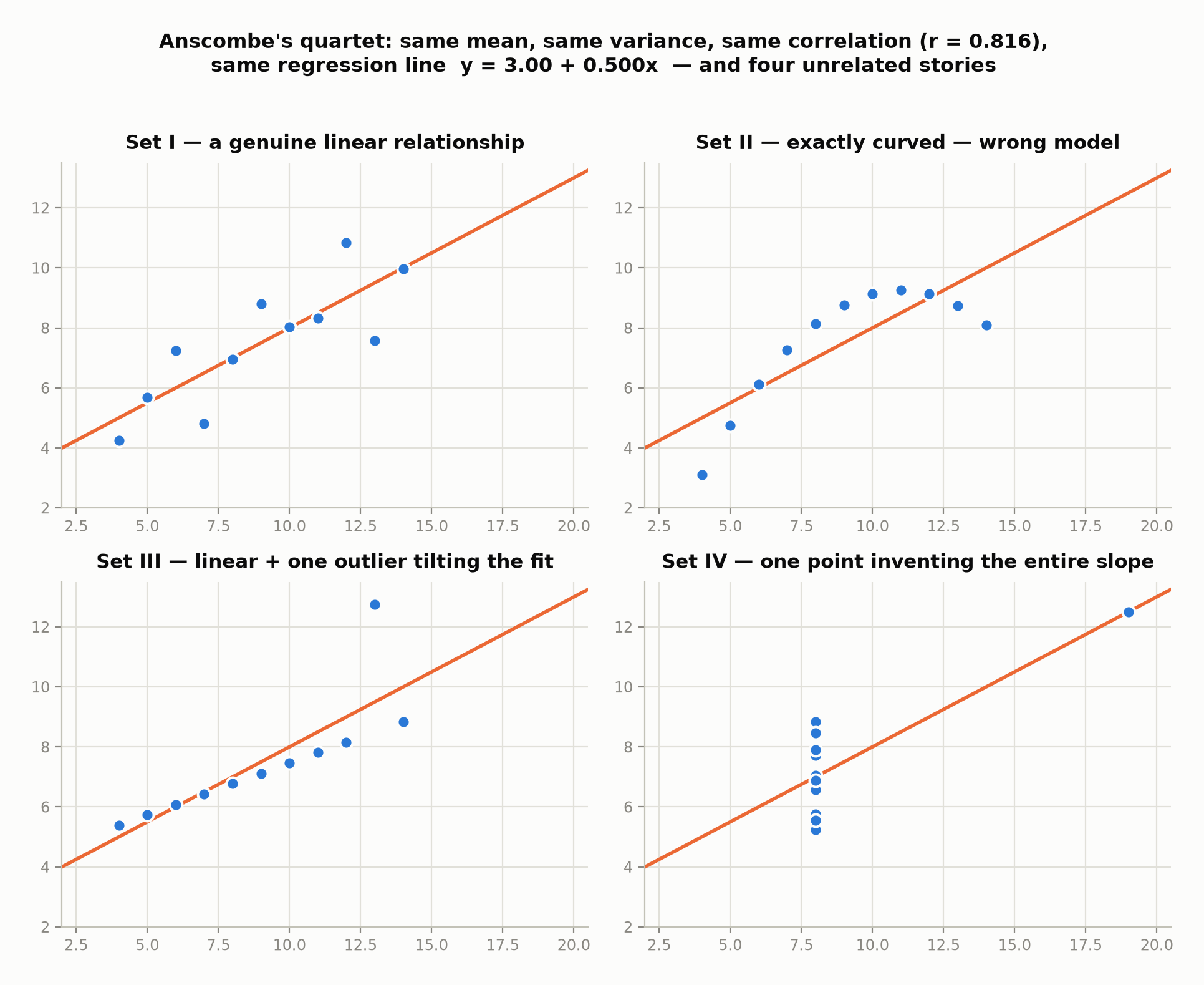
Set II is the one worth dwelling on: its R^2 = 0.67 is unremarkable, nothing in the summary table looks wrong, and the underlying relationship is a perfect parabola. No numeric check on this list would have caught it. Set IV is worse — ten points carry no information about the slope at all, and the eleventh decides it single-handedly.

Regression to the mean, simulated:

import numpy as np

rng = np.random.default_rng(0)
n = 100_000
skill = rng.normal(0, 1, n)
test1 = skill + rng.normal(0, 1, n)          # skill plus luck
test2 = skill + rng.normal(0, 1, n)          # same skill, new luck

top = test1 > np.quantile(test1, 0.95)       # the top 5% on test 1
print(f"top 5% on test 1: mean score {test1[top].mean():.4f}")
print(f"  their mean on test 2      : {test2[top].mean():.4f}")
print(f"  correlation between tests : {np.corrcoef(test1, test2)[0,1]:.4f}")
print("\nThey drop, on average -- not because they got worse, but because their")
print("test-1 score included good luck that doesn't repeat.")

Your turn

1. r = 0.8, s_x = 2, s_y = 6, \bar x = 10, \bar y = 50. Find the regression line.

2. A model has R^2 = 0.95. Does that mean it will predict well?

3. Why does spreading out the x values reduce \operatorname{SE}(\hat\beta_1)?

Solutions

1.

\hat\beta_1 = r\frac{s_y}{s_x} = 0.8 \times \frac{6}{2} = 2.4

\hat\beta_0 = \bar y - \hat\beta_1\bar x = 50 - 2.4(10) = 26

\hat y = 26 + 2.4x

Check: at x = \bar x = 10, \hat y = 26 + 24 = 50 = \bar y. ✓ The line passes through the point of means, as it must.

2. Not necessarily. R^2 is about variance explained, not prediction accuracy in useful units.

• If y has s_y = 1000, then R^2 = 0.95 leaves residual SD around \sqrt{0.05} \times 1000 \approx 224. Whether that's good depends entirely on what you need.
• R^2 is computed on the data you fit. Out-of-sample performance is usually worse, and a model with many predictors can have high R^2 purely from overfitting (§6, next lessons).
• A high R^2 with a systematically curved residual plot means the model is wrong even though it explains a lot — Anscombe's set II has R^2 = 0.67 and a perfect parabola underneath.

Better questions: what's \hat\sigma in the units I care about? What does the residual plot look like? How does it do on held-out data?

3. Because

\operatorname{SE}(\hat\beta_1) = \frac{\hat\sigma}{\sqrt{S_{xx}}}, \qquad S_{xx} = \sum(x_i - \bar x)^2

and spreading the x values out increases S_{xx} directly.

Geometrically: you're fitting a line, and a line is pinned down by how far apart its support points are. With all x values bunched together, a small wiggle in the data swings the slope wildly — you're extrapolating a direction from a short lever arm. Spread them out and the same wiggle barely tilts the line.

The design implication: if you can choose where to measure, measure at the extremes of the range you care about. For estimating a slope, two clusters at the ends beat an even spread. (For checking linearity, you want interior points too — otherwise a curve would go undetected.)

Check yourself in code

Fit the study-hours regression, verify the by-hand slope matches SciPy, and report R^2.

Print exactly this:

slope 4.0385
intercept 56.8077
R squared 0.9861
by hand matches: True

Round the slope and intercept to 4 decimal places and R^2 to 4.

import numpy as np
from scipy.stats import linregress

x = np.array([2, 3, 5, 7, 8], dtype=float)
y = np.array([65, 70, 75, 85, 90], dtype=float)

res = linregress(x, y)
print("slope", round(res.slope, 4))
print("intercept", round(res.intercept, 4))

# Print R squared, then recompute the slope by hand as Sxy / Sxx
# and confirm it matches.

import numpy as np
from scipy.stats import linregress

x = np.array([2, 3, 5, 7, 8], dtype=float)
y = np.array([65, 70, 75, 85, 90], dtype=float)

res = linregress(x, y)
print("slope", round(res.slope, 4))
print("intercept", round(res.intercept, 4))
print("R squared", round(res.rvalue**2, 4))

Sxx = ((x - x.mean()) ** 2).sum()
Sxy = ((x - x.mean()) * (y - y.mean())).sum()
print("by hand matches:", round(Sxy / Sxx, 4) == round(res.slope, 4))

---

Simple linear regression fits \hat y = \hat\beta_0 + \hat\beta_1 x by minimising squared residuals — which is maximum likelihood under Normal errors. The slope is the correlation rescaled into the units of the data, and because |r| \le 1, predictions always regress toward the mean. R^2 reports variance explained, and reports nothing about linearity, correctness, or causation.

Next: the same thing with many predictors, which is far cleaner in matrix form.