42. Model diagnostics

Fitting a regression is easy — lstsq always returns something. Deciding whether to believe it is the real work.

Every inference in the last two lessons rested on assumptions. This lesson is about checking them.

The assumptions, and what breaks

The mnemonic is LINE:

Assumption	If violated
Linearity: E[Y \mid x] really is linear	biased estimates, systematically wrong predictions
Independence of errors	standard errors wrong, usually far too small
Normality of errors	only matters for small-sample inference (CLT covers large n)
Equal variance (homoscedasticity)	estimates still unbiased, but standard errors wrong

Note the ordering of severity. Linearity and independence are the serious ones. Non-Normality is usually the least of your problems, despite getting the most attention.

Residual plots

Almost everything is visible in the residuals e_i = y_i - \hat y_i.

Residuals vs fitted values — the single most useful plot.

• Random scatter around zero → good.
• A curve → the relationship isn't linear. Add a quadratic term, transform, or use a different model.
• A funnel (spread growing with the fitted value) → heteroscedasticity.

These three are shapes, and shapes are worth seeing rather than reading about:

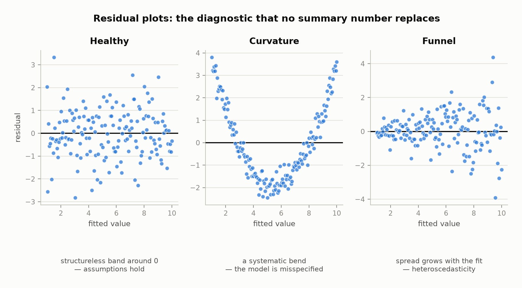
The middle and right panels are the reason this plot is worth drawing every time. Both models can report a perfectly respectable R^2; neither is trustworthy, and no single summary number on the fit would have told you.

Q-Q plot — residual quantiles against Normal quantiles. A straight line means Normal; curved ends mean heavy or light tails.

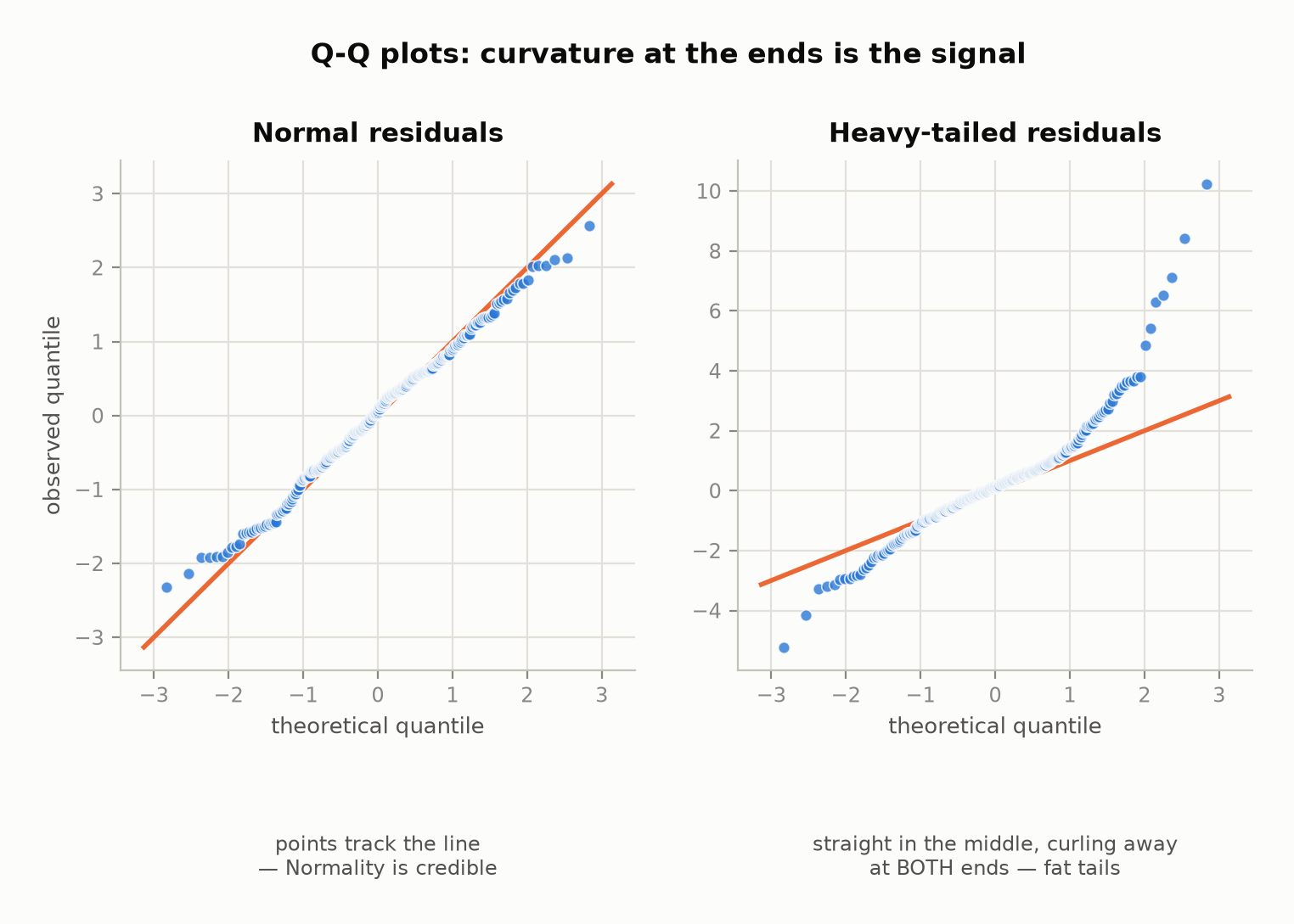
Note where the second plot goes wrong: the middle is fine. Tail problems are invisible in the bulk of the data, which is exactly why a Q-Q plot puts the quantiles on the axes instead of the values.

Residuals vs time or order — a visible pattern means autocorrelation, which violates independence.

Heteroscedasticity

Non-constant error variance. Common when y spans orders of magnitude — spending, income, counts — where the spread naturally grows with the level.

Consequences: \hat{\boldsymbol\beta} stays unbiased, but $\operatorname{Cov}(\hat{\boldsymbol\beta}) = \sigma^2(\mathbf X^\top\mathbf X)^{-1}$ is wrong, so every standard error, t-statistic, p-value and confidence interval is wrong.

Fixes:

• Transform the response (\log y is the usual first attempt).
• Robust (heteroscedasticity-consistent) standard errors — keep the same coefficients, compute honest standard errors. This is the standard modern fix.
• Weighted least squares, if you know the variance structure.

Multicollinearity

Predictors that are strongly correlated with each other. The signature, from the last lesson: a great fit with no significant coefficients, and unstable signs.

Measure it with the variance inflation factor:

\text{VIF}_j = \frac{1}{1 - R_j^2}

where R_j^2 comes from regressing x_j on all the other predictors. It says how much the variance of \hat\beta_j is inflated by the correlation.

• VIF = 1: uncorrelated with the others.
• VIF > 5: worth attention.
• VIF > 10: serious.

A VIF of 10 means \operatorname{SE}(\hat\beta_j) is \sqrt{10} \approx 3.2 times larger than it would be with uncorrelated predictors.

Fixes: drop one of the correlated pair, combine them into an index, collect more data, or use ridge regression (two lessons on) — which is designed precisely for this.

Important: multicollinearity does not hurt prediction. If you only need \hat y, high VIFs are harmless. It damages interpretation of individual coefficients, which is a different goal.

Outliers, leverage and influence

Three distinct concepts that get conflated:

Outlier — a large residual. The model predicts it badly.

Leverage — an unusual x value. Measured by h_{ii}, the i-th diagonal of the hat matrix. Since \sum h_{ii} = p + 1, the average is (p+1)/n, and h_{ii} > 2(p+1)/n is the usual flag.

Influence — the point actually changes the fit. This needs both high leverage and a large residual. Measured by Cook's distance:

D_i = \frac{e_i^2}{(p+1)\hat\sigma^2}\cdot\frac{h_{ii}}{(1-h_{ii})^2}

with D_i > 1 a common threshold.

The distinction matters. A point far out in x that sits exactly on the trend has high leverage and no influence — it's helping. A point in the middle of the x range with a big residual is an outlier with little influence. Only the combination moves the line.

Never delete points just because they're outliers. Investigate first: data error, a different population, or a genuine extreme value? Deleting inconvenient data is how you get results that don't replicate.

Worked example

Data with an influential point:

x: 1, 2, 3, 4, 5, 20 y: 2, 4, 6, 8, 10, 12

The first five points lie exactly on y = 2x. The sixth breaks the pattern — and sits far out in x.

With all six points, least squares gives \hat y = 4.56 + 0.42x.

With the first five only, it gives exactly \hat y = 0 + 2x.

One point has taken the slope from 2.00 to 0.42 — a 79% change — and pulled the intercept from 0 to 4.56.

Its leverage is h_{66} \approx 0.97, far above the 2(p+1)/n = 0.67 threshold, and Cook's distance is enormous. The point is dominating the fit essentially on its own.

What to do? Not "delete it". Find out what it is. If x = 20 is a typo for x = 2.0, fix it. If it's a genuine observation from a different regime, the honest answer is that a single straight line doesn't describe both regimes — and reporting the fit without mentioning it would be misleading either way.

Doing it in Python

Computing the diagnostics from scratch:

import numpy as np

x = np.array([1, 2, 3, 4, 5, 20], dtype=float)
y = np.array([2, 4, 6, 8, 10, 12], dtype=float)
X = np.column_stack([np.ones(len(x)), x])

n, k = X.shape
beta, *_ = np.linalg.lstsq(X, y, rcond=None)
H = X @ np.linalg.inv(X.T @ X) @ X.T
resid = y - X @ beta
h = np.diag(H)
sigma2 = (resid @ resid) / (n - k)
cooks = resid**2 / (k * sigma2) * h / (1 - h) ** 2

print("fit with all points:", beta.round(4))
beta5, *_ = np.linalg.lstsq(X[:5], y[:5], rcond=None)
print("fit without point 6:", beta5.round(4))

print(f"\n{'i':>3} {'x':>6} {'residual':>10} {'leverage':>10} {'Cook D':>10}")
for i in range(n):
    print(f"{i+1:>3} {x[i]:>6.1f} {resid[i]:>10.4f} {h[i]:>10.4f} {cooks[i]:>10.4f}")

print(f"\nleverage threshold 2(p+1)/n = {2*k/n:.4f}")
print(f"sum of leverages = {h.sum():.4f} (always p+1 = {k})")

Detecting heteroscedasticity, and the fix:

import numpy as np

rng = np.random.default_rng(0)
n = 300
x = rng.uniform(1, 10, n)
y = 2 + 3 * x + rng.normal(0, x, n)          # noise GROWS with x

X = np.column_stack([np.ones(n), x])
beta, *_ = np.linalg.lstsq(X, y, rcond=None)
resid = y - X @ beta

# The funnel, seen numerically: residual spread by quartile of fitted value
fitted = X @ beta
qs = np.quantile(fitted, [0, 0.25, 0.5, 0.75, 1.0])
print("residual spread across fitted-value quartiles:")
for lo, hi in zip(qs[:-1], qs[1:]):
    m = (fitted >= lo) & (fitted <= hi)
    print(f"  fitted in [{lo:6.2f}, {hi:6.2f}]: residual sd {resid[m].std():.3f}")

print("\nSpread grows steadily -> heteroscedastic.")

# Ordinary vs robust (White / HC0) standard errors
XtX_inv = np.linalg.inv(X.T @ X)
se_ols = np.sqrt(np.diag((resid @ resid) / (n - 2) * XtX_inv))
meat = X.T @ np.diag(resid**2) @ X
se_robust = np.sqrt(np.diag(XtX_inv @ meat @ XtX_inv))

print(f"\n{'term':>10} {'OLS se':>10} {'robust se':>12} {'ratio':>8}")
for name, a, b in zip(["intercept", "slope"], se_ols, se_robust):
    print(f"{name:>10} {a:>10.4f} {b:>12.4f} {b/a:>8.3f}")
print("\nOLS standard errors are too small here -- the robust ones are honest.")

VIF, and the proof that collinearity doesn't hurt prediction:

import numpy as np

rng = np.random.default_rng(1)
n = 200
x1 = rng.normal(0, 1, n)
x2 = x1 + rng.normal(0, 0.1, n)               # nearly identical to x1
x3 = rng.normal(0, 1, n)                      # independent
y = 2 + 1.5 * x1 + 0.5 * x2 + 3 * x3 + rng.normal(0, 1, n)

def vif(X, j):
    others = np.delete(X, j, axis=1)
    A = np.column_stack([np.ones(len(X)), others])
    b, *_ = np.linalg.lstsq(A, X[:, j], rcond=None)
    r = X[:, j] - A @ b
    return 1 / (1 - (1 - (r @ r) / ((X[:, j] - X[:, j].mean()) ** 2).sum()))

P = np.column_stack([x1, x2, x3])
for j, name in enumerate(["x1", "x2", "x3"]):
    print(f"VIF({name}) = {vif(P, j):8.2f}")

X = np.column_stack([np.ones(n), P])
beta, *_ = np.linalg.lstsq(X, y, rcond=None)
resid = y - X @ beta
se = np.sqrt(np.diag((resid @ resid) / (n - 4) * np.linalg.inv(X.T @ X)))
print(f"\n{'term':>10} {'estimate':>10} {'std err':>10}")
for name, b, s in zip(["intercept", "x1", "x2", "x3"], beta, se):
    print(f"{name:>10} {b:>10.4f} {s:>10.4f}")

print(f"\nR^2 = {1 - (resid@resid)/((y-y.mean())**2).sum():.4f}")
print("x1 and x2 have huge standard errors; x3 is estimated precisely.")
print("But the model still PREDICTS well -- collinearity hurts interpretation only.")

Curvature that R^2 won't tell you about:

import numpy as np

rng = np.random.default_rng(2)
n = 200
x = np.linspace(-3, 3, n)
y = x**2 + rng.normal(0, 0.5, n)             # genuinely quadratic

X = np.column_stack([np.ones(n), x])
beta, *_ = np.linalg.lstsq(X, y, rcond=None)
resid = y - X @ beta

print(f"linear fit R^2 = {1 - (resid@resid)/((y-y.mean())**2).sum():.4f}")
print("\nmean residual by region of x:")
for lo, hi in [(-3, -1.5), (-1.5, 0), (0, 1.5), (1.5, 3)]:
    m = (x >= lo) & (x < hi)
    print(f"  x in [{lo:>5}, {hi:>4}): mean residual {resid[m].mean():+.4f}")

print("\nPositive, negative, negative, positive -- a clear U shape in the residuals.")
print("The model is wrong, and no single R^2 number would have told you.")

Your turn

1. Residuals fan out as fitted values grow. What's wrong, and what would you do?

2. A predictor has VIF = 15. Is this always a problem?

3. A point has high leverage but a tiny residual. Is it influential?

Solutions

1. That's heteroscedasticity — the error variance grows with the mean.

The coefficients are still unbiased, but the standard errors are wrong, so the p-values and confidence intervals can't be trusted. With a fanning pattern they're typically too small, making results look more significant than they are.

Fixes, roughly in order of what to try:

• Transform y — \log y or \sqrt y often stabilises variance when the spread is proportional to the level. This also frequently fixes non-linearity at the same time.
• Robust standard errors — keep the fit, correct the inference. The usual choice when you want to keep y on its original scale.
• Weighted least squares — if you know the variance structure, weight by its reciprocal.

2. No — it depends what you want the model for.

If you're predicting, high VIF is harmless. The fitted values and their intervals are unaffected; only the split of credit between correlated predictors is unstable.

If you're interpreting individual coefficients, VIF = 15 is a real problem: \operatorname{SE}(\hat\beta_j) is inflated by \sqrt{15} \approx 3.9, so the coefficient is nearly uninterpretable and may well flip sign in a new sample.

Also worth knowing: a high VIF on a control variable you don't intend to interpret doesn't matter. And VIFs computed on polynomial or interaction terms are routinely large by construction — centring the predictors usually removes that artefact.

3. No.

Influence requires both an unusual x (leverage) and a poorly-fitted y (large residual). Cook's distance multiplies the two:

D_i = \frac{e_i^2}{(p+1)\hat\sigma^2}\cdot\frac{h_{ii}}{(1-h_{ii})^2}

If e_i \approx 0, then D_i \approx 0 no matter how large h_{ii} is.

Intuitively: a point far out in x that lands exactly on the line is confirming the trend, not distorting it. In fact it's helping — remember \operatorname{SE}(\hat\beta_1) = \hat\sigma/\sqrt{S_{xx}}, so a distant x value increases S_{xx} and makes the slope more precise.

The dangerous combination is high leverage plus a large residual — that's the x = 20 point in the worked example, which single-handedly rewrote the fit.

Check yourself in code

Compute the diagnostics for the influential-point example: show how much the slope changes when the point is dropped, and confirm it has high leverage.

Print exactly this:

slope with all 6 0.4186
slope without 2.0
leverage of point 6 0.9668
above threshold: True

Round the slopes to 4 decimal places and the leverage to 4. The leverage threshold is 2(p+1)/n.

import numpy as np

x = np.array([1, 2, 3, 4, 5, 20], dtype=float)
y = np.array([2, 4, 6, 8, 10, 12], dtype=float)
X = np.column_stack([np.ones(len(x)), x])

beta, *_ = np.linalg.lstsq(X, y, rcond=None)
print("slope with all 6", round(beta[1], 4))

# Refit without the last point, then compute the hat matrix and report
# the leverage of point 6 against the 2(p+1)/n threshold.

import numpy as np

x = np.array([1, 2, 3, 4, 5, 20], dtype=float)
y = np.array([2, 4, 6, 8, 10, 12], dtype=float)
X = np.column_stack([np.ones(len(x)), x])

beta, *_ = np.linalg.lstsq(X, y, rcond=None)
print("slope with all 6", round(beta[1], 4))

beta5, *_ = np.linalg.lstsq(X[:5], y[:5], rcond=None)
print("slope without", round(beta5[1], 4))

H = X @ np.linalg.inv(X.T @ X) @ X.T
h = np.diag(H)
print("leverage of point 6", round(h[-1], 4))

n, k = X.shape
print("above threshold:", bool(h[-1] > 2 * k / n))

---

Fitting is not checking. Residuals versus fitted values catches non-linearity and heteroscedasticity; Q-Q plots catch tail problems; VIFs catch collinearity; leverage and Cook's distance catch points that are rewriting the fit on their own. Linearity and independence are the assumptions worth worrying about most — and non-Normality the least.

Next: what to do when the response isn't continuous at all.