Ridge and lasso regularization · Probability & Statistics

Least squares is BLUE — the best linear unbiased estimator (§6). But §4 showed that unbiasedness is a convention, not a virtue, and that accepting some bias can cut variance enough to lower the total error.

Regularization does exactly that, deliberately.

The problem

Ordinary least squares struggles when:

p is close to n — the model has enough freedom to chase noise.
p > n — \mathbf{X}^\top\mathbf{X} is singular; no unique solution exists at all.
Predictors are collinear — coefficients become huge, unstable, and flip sign between samples (§6, lesson 2).

The common symptom is enormous coefficients: large positive and negative values nearly cancelling. The fit is excellent in-sample and terrible out-of-sample. That's overfitting.

The idea: penalise size

Add a penalty on the coefficients to the objective:

$\text{minimise} \quad \underbrace{\|\mathbf y - \mathbf X\boldsymbol\beta\|^2}_{\text{fit}} + \underbrace{\lambda \cdot \text{penalty}(\boldsymbol\beta)}_{\text{complexity}}$

\lambda \ge 0 controls the trade-off:

\lambda = 0 → ordinary least squares.
\lambda \to \infty → all coefficients driven to zero.
In between → shrinkage.

Ridge regression (L2)

$\hat{\boldsymbol\beta}_{\text{ridge}} = \arg\min \|\mathbf y - \mathbf X\boldsymbol\beta\|^2 + \lambda\sum_{j=1}^p \beta_j^2$

This has a closed form:

$\hat{\boldsymbol\beta}_{\text{ridge}} = (\mathbf X^\top\mathbf X + \lambda\mathbf I)^{-1}\mathbf X^\top\mathbf y$

Compare with OLS: the only change is +\lambda\mathbf I on the diagonal. That single addition makes the matrix invertible even when \mathbf X^\top\mathbf X is singular — which is why ridge works with p > n and with perfectly collinear predictors.

Properties:

Shrinks all coefficients toward zero, but never exactly to zero.
Handles collinearity gracefully: correlated predictors get similar shrunken coefficients rather than wild opposing ones.
Keeps every predictor in the model.

Lasso (L1)

$\hat{\boldsymbol\beta}_{\text{lasso}} = \arg\min \|\mathbf y - \mathbf X\boldsymbol\beta\|^2 + \lambda\sum_{j=1}^p |\beta_j|$

Swapping squares for absolute values changes the behaviour qualitatively:

Sets coefficients exactly to zero — so it performs variable selection automatically.
No closed form; solved by coordinate descent or LARS.
With correlated predictors it tends to pick one arbitrarily and zero the rest.

Why L1 zeroes things and L2 doesn't

The geometric argument is the clearest.

The constraint region for L2 is a circle (\sum\beta_j^2 \le t); for L1 it's a diamond (\sum|\beta_j| \le t). The solution is where the elliptical contours of the squared-error surface first touch that region.

A diamond has corners on the axes, and a corner is where some coefficient is exactly zero. Contours are overwhelmingly likely to touch a corner first. A circle has no corners — contact is generically at a point with all coordinates non-zero.

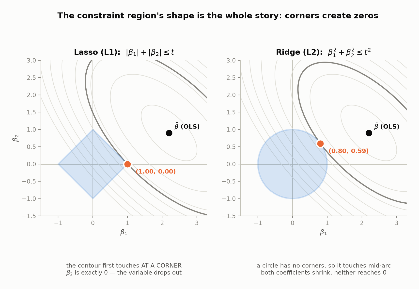
Both panels use the same data and the same budget t; only the shape of the constraint changes. The lasso solution lands on the corner with \beta_2 = 0 exactly — not 0.004, exactly zero — while ridge lands mid-arc with both coefficients merely smaller. The emphasised contour in each panel is the one that actually touches, so you can see the tangency rather than take it on trust.

Equivalently, in calculus terms: |\beta| has a non-differentiable kink at zero, which creates a range of gradients where zero stays optimal. \beta^2 has derivative zero at the origin, so there's no such flat spot.

Elastic net

Combine both:

$\lambda\left(\alpha\sum|\beta_j| + \frac{1-\alpha}{2}\sum\beta_j^2\right)$

Gets the sparsity of lasso plus ridge's handling of correlated groups — with correlated predictors it selects or drops them together, where lasso picks one at random.

Two practical necessities

1. Standardise the predictors. The penalty is on the raw coefficient magnitudes, so a predictor measured in millimetres would get a coefficient 1000× larger than the same predictor in metres, and be penalised 1000× (or 10^6×) harder. Always centre and scale before fitting.

2. Don't penalise the intercept. Otherwise the model isn't invariant to shifting y — adding 100 to every response would change the fit in a way that has nothing to do with complexity. Standard software excludes it automatically.

Choosing \lambda

By cross-validation, essentially always:

Split the data into k folds.
For each candidate \lambda: fit on k-1 folds, measure error on the held- out fold, average over folds.
Pick the \lambda minimising average validation error.

A common refinement is the one-standard-error rule: choose the largest \lambda whose error is within one standard error of the minimum. This gives a simpler model at almost no cost in accuracy.

Never choose \lambda on the training error — it's monotone in \lambda and would always pick 0.

The bias–variance picture

As \lambda increases: bias rises, variance falls. Test error is U-shaped, and its minimum is generally at some \lambda > 0.

That minimum sits at a biased estimator. It's the concrete pay-off of §4's MSE decomposition — trading a little bias for a lot of variance reduction genuinely wins, and Gauss–Markov doesn't contradict it because ridge isn't unbiased.

Worked example

20 observations, 30 predictors, only 3 of which matter.

With p > n there is no unique least squares solution at all — the model has more freedom than the data can constrain.

OLS: the training MSE is exactly 0.0. The fit passes through every single point, because with 30 free coefficients and 20 observations it can. That is pure memorisation, and the test MSE of 7.10 shows it — against a noise variance of 1, the model is roughly seven times worse than it should be.

Ridge at \lambda = 1: coefficients shrink, the training error rises to 0.047 — the fit is now deliberately imperfect — and the test MSE falls to 6.65.

Lasso: zeroes out most of the irrelevant predictors, keeping a handful — often recovering close to the true sparse structure, and giving a model you can actually read.

Two things are worth noticing about these numbers. The improvement from ridge is real but modest (7.10 → 6.65), because NumPy's lstsq already returns the minimum-norm solution when the system is underdetermined, which is itself a mild form of regularization. And training error moved in the opposite direction to test error — which is precisely why \lambda can never be chosen by looking at the fit.

The code below runs exactly this.

Doing it in Python

Ridge from the closed form, showing the shrinkage path:

import numpy as np

rng = np.random.default_rng(0)
n, p = 20, 30
X = rng.normal(0, 1, (n, p))
true_beta = np.zeros(p)
true_beta[:3] = [3.0, -2.0, 1.5]           # only 3 predictors matter
y = X @ true_beta + rng.normal(0, 1, n)

def ridge(X, y, lam):
    return np.linalg.solve(X.T @ X + lam * np.eye(X.shape[1]), X.T @ y)

print(f"{'lambda':>10} {'||beta||':>10} {'max |beta|':>12} {'train MSE':>12}")
for lam in (0.0, 0.1, 1.0, 10.0, 100.0):
    try:
        b = ridge(X, y, lam)
    except np.linalg.LinAlgError:
        print(f"{lam:>10} singular")
        continue
    resid = y - X @ b
    print(f"{lam:>10} {np.linalg.norm(b):>10.4f} {np.abs(b).max():>12.4f} "
          f"{(resid @ resid) / n:>12.6f}")

print("\nTraining error only ever increases with lambda -- which is why you")
print("cannot choose lambda by looking at it.")

The honest comparison, on held-out data:

import numpy as np

rng = np.random.default_rng(0)
n, p = 20, 30
X = rng.normal(0, 1, (n, p))
true_beta = np.zeros(p)
true_beta[:3] = [3.0, -2.0, 1.5]
y = X @ true_beta + rng.normal(0, 1, n)

X_test = rng.normal(0, 1, (500, p))
y_test = X_test @ true_beta + rng.normal(0, 1, 500)

def ridge(X, y, lam):
    return np.linalg.solve(X.T @ X + lam * np.eye(X.shape[1]), X.T @ y)

ols = np.linalg.lstsq(X, y, rcond=None)[0]
print(f"{'model':>16} {'train MSE':>12} {'test MSE':>12} {'||beta||':>10}")
for name, b in [("OLS", ols)] + [(f"ridge lam={l}", ridge(X, y, l)) for l in (1.0, 5.0)]:
    tr = ((y - X @ b) ** 2).mean()
    te = ((y_test - X_test @ b) ** 2).mean()
    print(f"{name:>16} {tr:>12.4f} {te:>12.4f} {np.linalg.norm(b):>10.4f}")

print(f"\ntrue ||beta|| = {np.linalg.norm(true_beta):.4f}")
print("OLS fits the training data almost perfectly and generalises badly.")

Lasso by coordinate descent, showing the sparsity:

import numpy as np

def soft_threshold(z, gamma):
    return np.sign(z) * np.maximum(np.abs(z) - gamma, 0.0)

def lasso(X, y, lam, iters=1000):
    n, p = X.shape
    beta = np.zeros(p)
    norms = (X ** 2).sum(axis=0)
    for _ in range(iters):
        for j in range(p):
            resid = y - X @ beta + X[:, j] * beta[j]
            beta[j] = soft_threshold(X[:, j] @ resid, lam) / norms[j]
    return beta

rng = np.random.default_rng(0)
n, p = 20, 30
X = rng.normal(0, 1, (n, p))
true_beta = np.zeros(p)
true_beta[:3] = [3.0, -2.0, 1.5]
y = X @ true_beta + rng.normal(0, 1, n)

print(f"{'lambda':>8} {'non-zero':>10}  coefficients (first 6)")
for lam in (0.0, 1.0, 5.0, 20.0):
    b = lasso(X, y, lam)
    print(f"{lam:>8} {int((np.abs(b) > 1e-8).sum()):>10}  {np.round(b[:6], 3)}")

print(f"\ntruth      {int((true_beta != 0).sum()):>10}  {np.round(true_beta[:6], 3)}")
print("\nLasso drives coefficients to EXACTLY zero. Ridge never does.")

Cross-validation, done properly:

import numpy as np

rng = np.random.default_rng(1)
n, p = 60, 25
X = rng.normal(0, 1, (n, p))
true_beta = np.zeros(p)
true_beta[:4] = [2.0, -1.5, 1.0, 0.8]
y = X @ true_beta + rng.normal(0, 1, n)

def ridge(X, y, lam):
    return np.linalg.solve(X.T @ X + lam * np.eye(X.shape[1]), X.T @ y)

def cv_error(lam, k=5):
    folds = np.array_split(rng.permutation(n), k)
    errs = []
    for i in range(k):
        test_idx = folds[i]
        train_idx = np.concatenate([folds[j] for j in range(k) if j != i])
        b = ridge(X[train_idx], y[train_idx], lam)
        errs.append(((y[test_idx] - X[test_idx] @ b) ** 2).mean())
    return np.mean(errs)

lams = [0.01, 0.1, 1, 5, 10, 50, 100, 500]
errors = [cv_error(l) for l in lams]

print(f"{'lambda':>8} {'CV error':>12}")
for l, e in zip(lams, errors):
    mark = "  <- best" if e == min(errors) else ""
    print(f"{l:>8} {e:>12.4f}{mark}")

best = lams[int(np.argmin(errors))]
print(f"\nchosen lambda: {best}")

Your turn

1. Why does ridge work when p > n but OLS doesn't?

2. You want to identify which 5 of 100 predictors matter. Ridge or lasso?

3. What happens to bias and variance as \lambda increases?

Solutions

1. Because \mathbf X^\top\mathbf X + \lambda\mathbf I is always invertible for \lambda > 0, while \mathbf X^\top\mathbf X is not.

When p > n, the matrix \mathbf X^\top\mathbf X is p \times p but has rank at most n < p, so it's singular — infinitely many \boldsymbol\beta fit the data perfectly and OLS cannot choose among them.

Adding \lambda\mathbf I raises every eigenvalue by \lambda, so none are zero and the inverse exists. Equivalently: the penalty breaks the tie by picking the solution with the smallest norm among all perfect fits. The problem was never a shortage of solutions — it was a shortage of criteria.

2. Lasso.

Ridge shrinks every coefficient toward zero but leaves all 100 in the model, so it never tells you which ones matter — you'd still be reading 100 small numbers and guessing where to cut.

Lasso sets coefficients exactly to zero, performing variable selection as part of the fit. With a suitable \lambda it can recover a sparse model directly.

Two caveats worth knowing:

If some of the 100 predictors are highly correlated with each other, lasso picks one essentially arbitrarily. Elastic net is the better choice there, since it keeps correlated groups together.
The selected set is not a hypothesis test. Post-selection inference is a real and subtle problem — the p-values from refitting on the selected variables are not valid, because the selection used the same data.

3. As \lambda increases:

Bias increases. Coefficients are pulled toward zero and away from their true values. At \lambda \to \infty every coefficient is 0 and the bias is maximal.
Variance decreases. The fit is less free to chase noise, so it changes less between samples. At \lambda \to \infty the variance is 0 — the model always predicts \bar y.

Since \operatorname{MSE} = \operatorname{Var} + \text{Bias}^2, the total is U-shaped in \lambda, and its minimum is generally at some \lambda > 0.

That's the entire justification: a biased estimator beating the unbiased one on total error. Gauss–Markov isn't violated — it only claims OLS is best among unbiased estimators, and ridge deliberately leaves that class.

Check yourself in code

Compare OLS against ridge on data with more predictors than the sample can support, using held-out test data.

Print exactly this:

OLS train MSE 0.0
OLS test MSE 7.1006
ridge test MSE 6.6512
ridge wins: True

Use default_rng(0), n = 20, p = 30, true coefficients [3, -2, 1.5] then zeros, noise sd 1, a test set of 500, and \lambda = 1. Round every MSE to 4 decimal places.

import numpy as np

rng = np.random.default_rng(0)
n, p = 20, 30
X = rng.normal(0, 1, (n, p))
true_beta = np.zeros(p)
true_beta[:3] = [3.0, -2.0, 1.5]
y = X @ true_beta + rng.normal(0, 1, n)

X_test = rng.normal(0, 1, (500, p))
y_test = X_test @ true_beta + rng.normal(0, 1, 500)

ols = np.linalg.lstsq(X, y, rcond=None)[0]
print("OLS train MSE", round(((y - X @ ols) ** 2).mean(), 4))

# Print the OLS test MSE, then fit ridge with lambda = 1 using
# solve(X.T @ X + lam * I, X.T @ y) and compare test MSEs.

import numpy as np

rng = np.random.default_rng(0)
n, p = 20, 30
X = rng.normal(0, 1, (n, p))
true_beta = np.zeros(p)
true_beta[:3] = [3.0, -2.0, 1.5]
y = X @ true_beta + rng.normal(0, 1, n)

X_test = rng.normal(0, 1, (500, p))
y_test = X_test @ true_beta + rng.normal(0, 1, 500)

ols = np.linalg.lstsq(X, y, rcond=None)[0]
print("OLS train MSE", round(((y - X @ ols) ** 2).mean(), 4))

ols_test = ((y_test - X_test @ ols) ** 2).mean()
print("OLS test MSE", round(ols_test, 4))

lam = 1.0
ridge = np.linalg.solve(X.T @ X + lam * np.eye(p), X.T @ y)
ridge_test = ((y_test - X_test @ ridge) ** 2).mean()
print("ridge test MSE", round(ridge_test, 4))
print("ridge wins:", bool(ridge_test < ols_test))

Regularization adds a penalty on coefficient size, deliberately trading bias for variance. Ridge (L2) shrinks smoothly, handles collinearity, and works even when p > n because +\lambda\mathbf I makes the matrix invertible. Lasso (L1) shrinks and selects, driving coefficients exactly to zero because its constraint region has corners. Standardise first, don't penalise the intercept, and choose \lambda by cross-validation.

That closes §6. Next: a different philosophy of inference entirely — treating the parameter itself as a random variable.

44. Ridge and lasso regularization