63. Mutual information
Correlation (§2) measures linear association, and we saw it miss a perfect parabola entirely. Mutual information measures association of any kind.
The definition
I(X; Y) = D_{KL}\big(p(x,y) \parallel p(x)p(y)\big) = \sum_{x,y}p(x,y)\log\frac{p(x,y)}{p(x)p(y)}
It is the KL divergence between the joint distribution and what the joint would be if X and Y were independent.
So it measures how far the pair is from independence — and since independence is exactly p(x,y) = p(x)p(y) (§2), the connection is immediate:
I(X; Y) = 0 \iff X \perp Y
Not "uncorrelated" — genuinely independent. That is the whole advantage over correlation.
Equivalent forms
I(X;Y) = H(X) - H(X \mid Y) = H(Y) - H(Y \mid X)
I(X;Y) = H(X) + H(Y) - H(X,Y)
The first is the one to internalise: mutual information is the reduction in uncertainty about X from learning Y. It's the number of bits Y tells you about X.
The second shows it as an overlap — the shared part of the two entropies, which is why the standard picture is a Venn diagram of H(X) and H(Y) with I(X;Y) as the intersection:
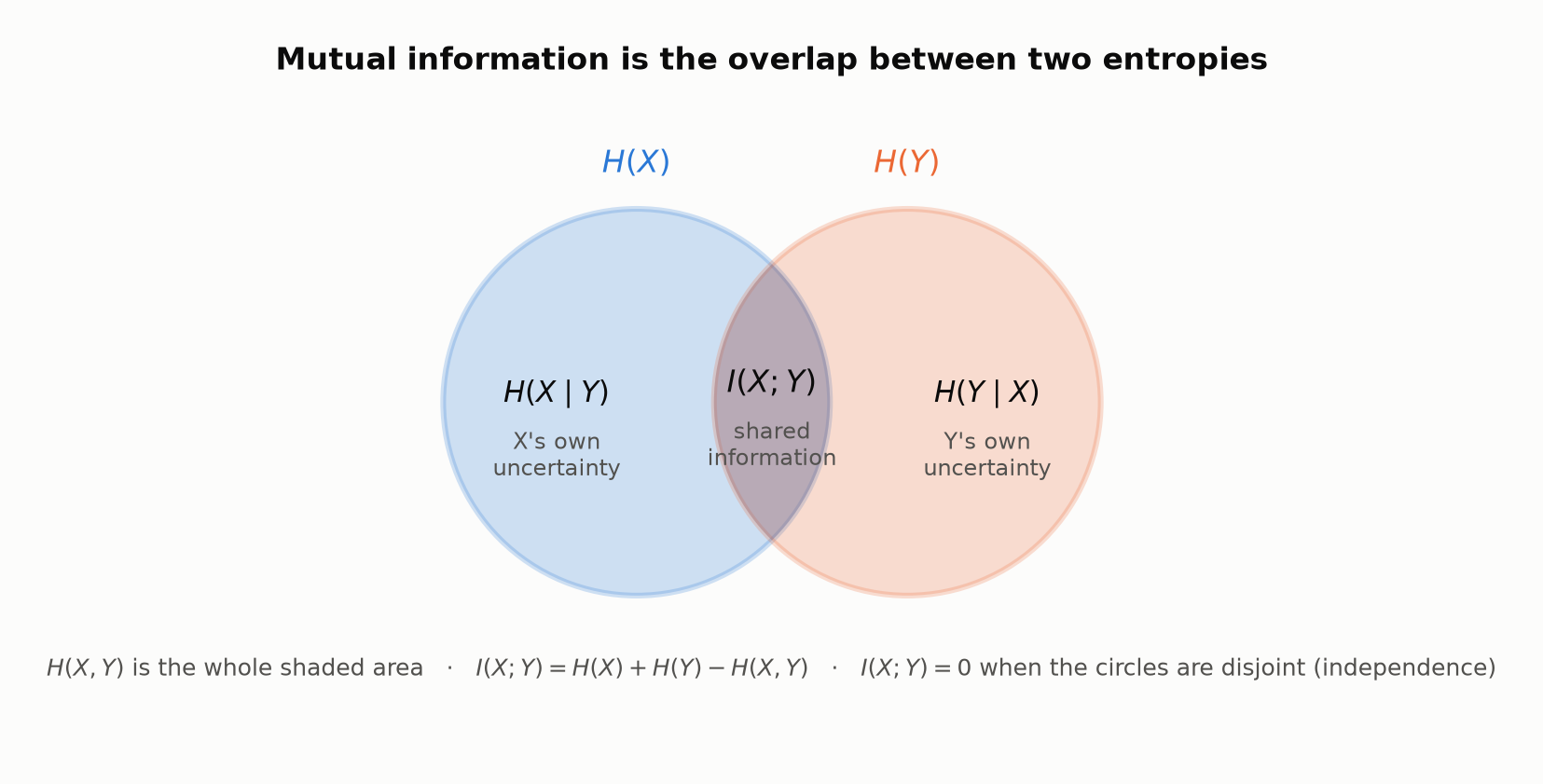
Read the picture and the identities fall out of it. H(X) - H(X \mid Y) is the left circle minus its left-only crescent — the intersection. Independence is the case where the circles pull apart entirely, leaving I(X;Y) = 0 and H(X,Y) = H(X) + H(Y).
One caution about this picture: it is exact for two variables and starts lying for three, where the "triple intersection" I(X;Y;Z) can be negative — an area no Venn diagram can draw. Trust it here; don't extrapolate it.
Properties
Non-negative: I(X;Y) \ge 0 — it's a KL divergence. Learning something can never, on average, increase your uncertainty.
Symmetric: I(X;Y) = I(Y;X). Despite being built from an asymmetric divergence, the symmetry of the joint makes it symmetric. This is why mutual information is usable as a similarity measure where KL is not.
Bounded: I(X;Y) \le \min\big(H(X), H(Y)\big), with equality when one variable determines the other.
Self-information: I(X;X) = H(X) — a variable tells you everything about itself.
Invariant under invertible transformations. I(f(X); g(Y)) = I(X;Y) for invertible f, g. Correlation has nothing like this: it changes under any nonlinear transformation. Mutual information doesn't care what units or encodings you use.
Versus correlation
Return to §2's counterexample: X uniform on \{-1, 0, 1\} and Y = X^2.
\rho(X, Y) = 0 \qquad \text{but} \qquad I(X;Y) > 0
Correlation sees nothing; mutual information sees the deterministic relationship. In fact I(X;Y) = H(Y), since X determines Y completely.
| Correlation | Mutual information | |
|---|---|---|
| Detects | linear only | any dependence |
| Range | [-1, 1] | [0, \min(H(X), H(Y))] |
| Zero means | uncorrelated | independent |
| Direction | sign shows it | no direction |
| Transformations | changes | invariant |
| Estimation from data | easy, stable | hard, especially continuous |
The catch is estimation. Correlation needs two moments and is stable in small samples. Mutual information needs the whole joint distribution, and estimating it from data is genuinely difficult — histogram-based estimators are biased upward, reporting spurious dependence when bins are sparse. That bias is the single biggest practical pitfall, and the code below demonstrates it.
Uses
- Feature selection: rank features by I(\text{feature}; \text{target}), catching nonlinear relationships that correlation filters would discard.
- Channel capacity: Shannon's noisy-channel theorem defines capacity as \max_{p(x)} I(X;Y) — the maximum reliable transmission rate.
- Decision trees: information gain at a split is exactly the mutual information between the feature and the label.
- Representation learning: objectives like InfoMax maximise I between inputs and learned representations.
- Independence testing: a nonparametric alternative to \chi^2.
Worked example
Joint distribution of X (rows) and Y (columns):
| Y=0 | Y=1 | |
|---|---|---|
| X=0 | 0.4 | 0.1 |
| X=1 | 0.1 | 0.4 |
Marginals: p_X = (0.5, 0.5), p_Y = (0.5, 0.5), so H(X) = H(Y) = 1 bit.
Joint entropy:
H(X,Y) = -(0.4\log_2 0.4 \times 2 + 0.1\log_2 0.1 \times 2) = 2(0.529) + 2(0.332) = 1.722 \text{ bits}
Mutual information:
I(X;Y) = H(X) + H(Y) - H(X,Y) = 1 + 1 - 1.722 = 0.278 \text{ bits}
Interpretation: knowing Y reduces your uncertainty about X by 0.278 of the 1 bit you started with — a bit over a quarter of it.
That matches intuition: the variables agree 80% of the time, so Y is informative but far from decisive. If they agreed always, H(X,Y) would be 1 and I would be the full 1 bit. If they were independent, H(X,Y) would be 2 and I would be 0.
Compare with correlation: here \rho = 0.6, and both measures agree there's a real association. They only diverge when the relationship is nonlinear.
Doing it in Python
Mutual information from a joint table, three equivalent ways:
import numpy as np

def H(p):
    p = np.asarray(p, float).ravel()
    p = p[p > 0]
    return -np.sum(p * np.log2(p))

def mutual_information(joint):
    joint = np.asarray(joint, float)
    px, py = joint.sum(axis=1), joint.sum(axis=0)
    return H(px) + H(py) - H(joint)

joint = np.array([[0.4, 0.1],
                  [0.1, 0.4]])
px, py = joint.sum(axis=1), joint.sum(axis=0)

print(f"H(X)   = {H(px):.4f}")
print(f"H(Y)   = {H(py):.4f}")
print(f"H(X,Y) = {H(joint):.4f}")
print(f"\nI(X;Y) = H(X) + H(Y) - H(X,Y) = {mutual_information(joint):.4f} bits")

# The KL form
kl_form = np.sum(joint * np.log2(joint / np.outer(px, py)))
print(f"I(X;Y) = KL(joint || product of marginals) = {kl_form:.4f} bits")

# The conditional-entropy form
h_x_given_y = sum(py[j] * H(joint[:, j] / py[j]) for j in range(2))
print(f"I(X;Y) = H(X) - H(X|Y) = {H(px) - h_x_given_y:.4f} bits")
Where mutual information beats correlation:
import numpy as np
from scipy.stats import pearsonr

def H(p):
    p = np.asarray(p, float).ravel()
    p = p[p > 0]
    return -np.sum(p * np.log2(p))

def mi_from_samples(x, y, bins=8):
    joint, _, _ = np.histogram2d(x, y, bins=bins)
    joint = joint / joint.sum()
    px, py = joint.sum(axis=1), joint.sum(axis=0)
    return H(px) + H(py) - H(joint)

rng = np.random.default_rng(0)
n = 20_000
x = rng.uniform(-3, 3, n)

relationships = {
    "independent":     rng.uniform(-3, 3, n),
    "linear":          2 * x + rng.normal(0, 0.5, n),
    "quadratic":       x**2 + rng.normal(0, 0.5, n),
    "sine":            np.sin(3 * x) + rng.normal(0, 0.1, n),
    "deterministic":   x.copy(),
}
print(f"{'relationship':>16} {'|correlation|':>15} {'mutual info':>13}")
for name, y in relationships.items():
    r = abs(pearsonr(x, y)[0])
    print(f"{name:>16} {r:>15.4f} {mi_from_samples(x, y):>13.4f}")

print("\nQuadratic and sine have near-zero correlation but high mutual")
print("information -- exactly the dependence correlation cannot see.")
The estimation bias — the biggest practical trap:
import numpy as np

def H(p):
    p = np.asarray(p, float).ravel()
    p = p[p > 0]
    return -np.sum(p * np.log2(p))

def mi_from_samples(x, y, bins):
    joint, _, _ = np.histogram2d(x, y, bins=bins)
    joint = joint / joint.sum()
    px, py = joint.sum(axis=1), joint.sum(axis=0)
    return H(px) + H(py) - H(joint)

rng = np.random.default_rng(1)

print("TRUE mutual information is 0 -- the variables are independent.\n")
print(f"{'n':>8} {'4 bins':>10} {'10 bins':>10} {'30 bins':>10}")
for n in (50, 200, 1_000, 10_000, 100_000):
    x, y = rng.uniform(size=n), rng.uniform(size=n)
    row = [mi_from_samples(x, y, b) for b in (4, 10, 30)]
    print(f"{n:>8} {row[0]:>10.4f} {row[1]:>10.4f} {row[2]:>10.4f}")

print("\nEvery estimate is positive despite the truth being 0. The bias grows")
print("with the number of bins and shrinks with n -- never trust a small-sample")
print("mutual information without a permutation test.")
The fix: a permutation test that calibrates against the bias:
import numpy as np

def H(p):
    p = np.asarray(p, float).ravel()
    p = p[p > 0]
    return -np.sum(p * np.log2(p))

def mi(x, y, bins=8):
    joint, _, _ = np.histogram2d(x, y, bins=bins)
    joint = joint / joint.sum()
    return H(joint.sum(axis=1)) + H(joint.sum(axis=0)) - H(joint)

rng = np.random.default_rng(2)
n = 500

for label, y_builder in [
    ("independent", lambda x: rng.uniform(-3, 3, n)),
    ("quadratic",   lambda x: x**2 + rng.normal(0, 0.5, n)),
]:
    x = rng.uniform(-3, 3, n)
    y = y_builder(x)
    observed = mi(x, y)
    null = np.array([mi(x, rng.permutation(y)) for _ in range(300)])
    pval = (null >= observed).mean()
    print(f"{label:>14}: MI = {observed:.4f}, null mean = {null.mean():.4f}, "
          f"p = {pval:.4f}")

print("\nShuffling destroys any real dependence while KEEPING the bias,")
print("so the permutation distribution is the honest baseline to compare against.")
Your turn
1. I(X;X) = ?
2. If X and Y are independent, what is I(X;Y)?
3. Why can mutual information detect relationships that correlation misses?
Solutions
1. I(X;X) = H(X).
From I(X;Y) = H(X) - H(X \mid Y) with Y = X:
I(X;X) = H(X) - H(X \mid X) = H(X) - 0 = H(X)
since knowing X leaves no uncertainty about X.
This is why H(X) is sometimes called the self-information: it's exactly how many bits X carries about itself. It also confirms the bound I(X;Y) \le \min(H(X), H(Y)) is tight — attained when one variable determines the other.
2. Zero.
Independence means p(x,y) = p(x)p(y), so the log term vanishes:
I(X;Y) = \sum_{x,y}p(x,y)\log\frac{p(x)p(y)}{p(x)p(y)} = \sum_{x,y}p(x,y)\log 1 = 0
Equivalently: I is the KL divergence between the joint and the product of marginals, and KL is zero exactly when its two arguments coincide (§10, lesson 3).
The converse also holds, and it's the important half: $I(X;Y) = 0 \implies X \perp Y$. Correlation has no such converse — zero correlation does not imply independence except for jointly Normal variables (§2).
3. Because it uses the whole joint distribution, not just second moments.
Correlation is built from E[XY] - E[X]E[Y] — a single number summarising linear co-movement. A relationship that is symmetric about the mean, like Y = X^2 with X symmetric, contributes positively on one side and negatively on the other, and the two cancel to exactly zero.
Mutual information compares p(x,y) against p(x)p(y) cell by cell. Any systematic deviation — in any direction, of any shape — contributes positively, because KL divergence is non-negative and vanishes only under exact equality. There is nothing to cancel.
The invariance property makes the same point structurally: $I(f(X); g(Y)) = I(X;Y)$ for invertible f, g. Dependence is a property of the joint distribution's structure, not of the particular coordinates you chose to express it in. Correlation is tied to the coordinates; mutual information isn't.
The cost, as noted, is estimation difficulty — and the code above shows how readily a naive histogram estimator invents dependence that isn't there.
Check yourself in code
Compute mutual information for a joint table three ways and confirm they agree.
Print exactly this:
H(X) 1.0
H(X,Y) 1.7219
I(X;Y) 0.2781
all three forms agree: True
Use the joint table [[0.4, 0.1], [0.1, 0.4]] with base-2 logarithms, rounded to 4 decimal places. The three forms are H(X)+H(Y)-H(X,Y), the KL divergence against the product of marginals, and H(X) - H(X \mid Y).
import numpy as np

def H(p):
    p = np.asarray(p, float).ravel()
    p = p[p > 0]
    return -np.sum(p * np.log2(p))

joint = np.array([[0.4, 0.1],
                  [0.1, 0.4]])
px, py = joint.sum(axis=1), joint.sum(axis=0)

print("H(X)", round(H(px), 4))
print("H(X,Y)", round(H(joint), 4))

# Compute I(X;Y) three ways and check they all match.
import numpy as np

def H(p):
    p = np.asarray(p, float).ravel()
    p = p[p > 0]
    return -np.sum(p * np.log2(p))

joint = np.array([[0.4, 0.1],
                  [0.1, 0.4]])
px, py = joint.sum(axis=1), joint.sum(axis=0)

print("H(X)", round(H(px), 4))
print("H(X,Y)", round(H(joint), 4))

form1 = H(px) + H(py) - H(joint)
form2 = np.sum(joint * np.log2(joint / np.outer(px, py)))
form3 = H(px) - sum(py[j] * H(joint[:, j] / py[j]) for j in range(2))

print("I(X;Y)", round(form1, 4))
print("all three forms agree:",
      round(form1, 4) == round(form2, 4) == round(form3, 4))
Mutual information is the KL divergence between a joint distribution and the product of its marginals, so it is zero exactly when two variables are independent — not merely uncorrelated. It's symmetric, invariant under invertible transformations, and reads as the number of bits one variable tells you about the other. Its weakness is estimation: naive estimators are biased upward, so calibrate against a permutation baseline.
That closes §10. Next: the computational methods that make all of this usable when the integrals have no closed form.